Including DOT Graphs as PostScript or PDF files in LaTeX documents

Graphviz is a great open source graph visualization software. In this post I’ll demonstrate how to include DOT graphs in PDF documents using LaTeX.

The most convenient way to insert graphics into PDF documents is to use vector graphics. In contrast to raster graphics (which are pixel-based) vector graphics can be scaled arbitrarily without getting “pixelated”.

From DOT the graphics can be exported in vector graphics as Portable Document Format (PDF) or Encapsulated Post Script (EPS) files. The file type you need depends on the LaTeX compiler you are using. The standard latex compiler can handle EPS files, whereas pdflatex supports PDF graphics.

Option 1: Using latex and EPS graphics

Assuming you have persisted your graph in a dot file, say myGraph.dot, you can convert it to an Encapsulated Post Script (EPS) file by using the dot tool from the command line:

1
dot -Tps2 myGraph.dot -o myGraph.eps

Here is a nice shell script which converts all dot files in the current directory to eps files:

1
2
3
4
5
6
7
8
#!/bin/bash
for f in *.dot; do
  basename=$(basename "$f")
  filename=${basename%.*}
  command="dot -Tps2 $f -o ${filename}.eps";
  echo $command;
  $command;
done

To use it, simply save it as an .sh file, execute chmod 755 on it and execute it in the terminal (works for unix-based systems only).

Having done that, we try to insert that image in our pdf file:

1
2
3
4
5
6
7
\begin{figure}[htp]
\begin{center}
  \includegraphics[width=0.9\textwidth]{myGraph}
  \caption{My Caption}
  \label{fig:myGraph}
\end{center}
\end{figure}

Note that the file extension is ommited.

Unfortunately, the pdflatex compiler does not support EPS images. But don’t worry, there are two options for solving that.

Option 2: Using pdflatex and PDF graphics

If you are using pdflatex, PDF graphics have to be produced instead of EPS graphics. This is done as described in the previous section, except another target file type is specified:

1
dot -Tpdf myGraph.dot -o myGraph.pdf

Option 3: Using pdflatex and converting EPS to PDF on the fly

The epstopdf LaTeX package converts your EPS files to PDF files on the fly, which then can be included in your document. This is how you must configure your graphic packages in the preamble of your LaTeX document (code from this blog post):

1
2
3
4
5
6
7
8
9
10
11
12
13
14
15
\newif\ifpdf
\ifx\pdfoutput\undefined
   \pdffalse
\else
   \pdfoutput=1
   \pdftrue
\fi
\ifpdf
   \usepackage{graphicx}
   \usepackage{epstopdf}
   \DeclareGraphicsRule{.eps}{pdf}{.pdf}{`epstopdf #1}
   \pdfcompresslevel=9
\else
   \usepackage{graphicx}
\fi

The epstopdf package will automatically create a PDF file of your figure and include it in your document. However, the following requirements must be fulfilled:

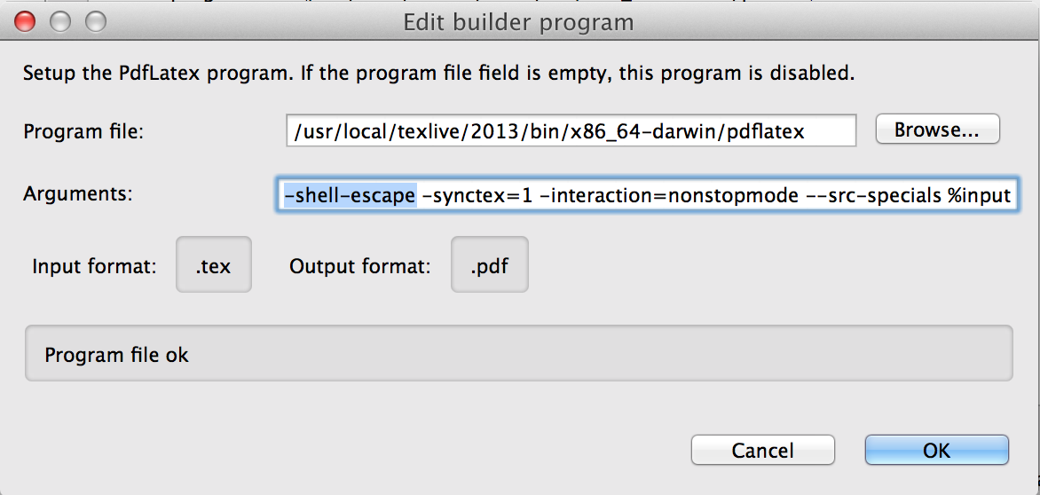
The -shell-escape option must be set when invoking the compiler. The command line setting for this invocation can be set in your LaTeX IDE. Here I will illustrate how to configure this setting using the TeXlipse IDE for Eclipse:

Builder SettingsOpen Preferences -> Texlipse -> Builder Settings, select the PdfLatex program and click Edit. The following dialog appears, in which you can add the -shell-escape option to the command line:

-shell-escape option
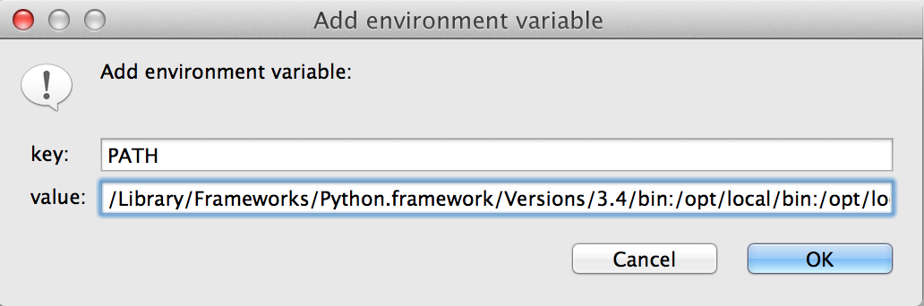
Another requirement (which is specific to the TeXlipse environment) is the PATH variable, which has to be set. Otherwise, the shell commands called from LaTeX can not be executed correctly. Check out your system path by opening a terminal and typing:

1
echo $PATH

Copy the output to the clipboard, and in TeXlipse go to Preferences -> TeXlipse -> Builder Settings -> Environment. Click Add and create a new environment variable named PATH with the value of your system path, which you just copied from the terminal:

AddEnvironmentVariableAfter that, the EPS-to-PDF conversion should work on the fly. If it does not work for some reason, you can manually invoke the conversion from the command line:

1
epstopdf myGraph.eps

You can now publish PDF documents with infinitely-scalable graphs 🙂

Defining Custom Language Templates for LaTeX Listings

The listings package enables LaTeX users to include source code snippets into LaTeX documents. The source code can be formatted using predefined languages templates. To select a predefined language, use the following code (as an example, Python is used):

\usepackage{listings}
\lstset{language=Python}
\lstinputlisting{path/to/myFile.py}

However, it is also possible to define own formatting templates for custom languages, which can be useful for developers of Domain-specific Languages (DSLs), for example. This is accomplished by using the command \lstdefinelanguage. The following example defines a language named myLang with various keywords, single line comments prefixed with //, multiline comments delimited by /* and */ and Strings delimited with double quotes:

% Define Language
\lstdefinelanguage{myLang}
{
  % list of keywords
  morekeywords={
    import,
    if,
    while,
    for
  },
  sensitive=false, % keywords are not case-sensitive
  morecomment=[l]{//}, % l is for line comment
  morecomment=[s]{/*}{*/}, % s is for start and end delimiter
  morestring=[b]" % defines that strings are enclosed in double quotes
}

Subsequently you can use the \lstset command to activate your language template for all following listings. All parameters are documented inline. This results in nice listings with line numbers, borders with rounded corners and syntax highlighting for comments, keywords and strings. The colors are based on the Java highlighting style in Eclipse:

% Define Colors
\usepackage{color}
\definecolor{eclipseBlue}{RGB}{42,0.0,255}
\definecolor{eclipseGreen}{RGB}{63,127,95}
\definecolor{eclipsePurple}{RGB}{127,0,85}
 
% Set Language
\lstset{
  language={myLang},
  basicstyle=\small\ttfamily, % Global Code Style
  captionpos=b, % Position of the Caption (t for top, b for bottom)
  extendedchars=true, % Allows 256 instead of 128 ASCII characters
  tabsize=2, % number of spaces indented when discovering a tab 
  columns=fixed, % make all characters equal width
  keepspaces=true, % does not ignore spaces to fit width, convert tabs to spaces
  showstringspaces=false, % lets spaces in strings appear as real spaces
  breaklines=true, % wrap lines if they don't fit
  frame=trbl, % draw a frame at the top, right, left and bottom of the listing
  frameround=tttt, % make the frame round at all four corners
  framesep=4pt, % quarter circle size of the round corners
  numbers=left, % show line numbers at the left
  numberstyle=\tiny\ttfamily, % style of the line numbers
  commentstyle=\color{eclipseGreen}, % style of comments
  keywordstyle=\color{eclipsePurple}, % style of keywords
  stringstyle=\color{eclipseBlue}, % style of strings
}

That’s it. Now you can include your listings in your custom language using

\lstinputlisting{path/to/myFile.ext}

Now have fun with your language and LaTeX 🙂

How to Install Custom LaTeX Extensions with MacTeX

When writing articles for conferences, authors are often supplied with custom layout templates, classes, bibliography styles etc. for LaTeX. The most common file extensions of these files are:

  • .cls – Class files to add new document classes
  • .bst – BibTeX Style files to format your bibliography
  • .sty – Style files containing LaTeX macros

Using those files documents are created according to the style guidelines of the conference proceedings / journals the article will be published in. When using MacTeX on Mac OS X, the proper location for custom extensions is:

~/Library/texmf/tex/latex/

where ~ ist your user home folder. I particularly needed this to install the LaTeX template for Springer Lecture Notes in Computer Science (LNCS), which are available here. After copying the whole llncs folder into ~/Library/texmf/tex/latex/, I could use the class in my LaTeX environment like this:

\documentclass{llncs}

Happy publishing 🙂

Installing LaTeX, Eclipse and TeXlipse on Mac OS X

LaTeX is an essential typesetting language for scientific papers and presentations. In this blog post I will explain how to install a complete LaTeX environment on your mac based on MacTex, Eclipse and TeXlipse. These components form a very powerful IDE for writing documents with LaTeX.

Installing a LaTeX distribution

The recommended LaTeX distribution to install on OS X is MacTex. Just follow the link, download the (very large!) installation bundle and execute it.

Installing Eclipse

Eclipse is a very powerful software platform, allowing to install plugins in order to assemble a flexible and powerful IDE. Download Eclipse (Version for Java Developers) here for your appropriate processor architecture. Unpack the file and execute Eclipse.app inside the unpacked folder.

If you are running Mountain Lion and get a system message that “Eclipse can not be executed because the developer is not verified”, unlock the App by starting a Terminal window and typing the following command:

xattr -d com.apple.quarantine /Applications/eclipse/Eclipse.app

Of course, you have to change the path to your custom location.

When Eclipse is started for the first time, it will ask you for a “workspace location”. This is a folder on your hard disk where your projects and files that are edited in Eclipse are stored. Choose an appropriate location of your choice and select “use this as default and do not ask again“.

01_workspace

On the first start, a welcome screen will appear, which you can simply close.

Installing TeXlipse (Option A – via Eclipse Marketplace)

To install the LaTeX plugin for Eclipse named TeXlipse, you simply go to Help -> Eclipse Marketplace.

03_marketplace

Wait until the list is loaded and type texlipse into the search field. TeXlipse will be listed as first option in the list. Click the Install button.

04_marketplace2

In the following dialog, click Next, read and accept the license and then click Finish. If you get a security warning saying that “you are trying to install software with unsigned content”, click OK. After the installation you’ll be asked to restart Eclipse, which you confirm with Yes.

Installing TeXlipse (Option B – Update Site)

If for some reason the menu item Eclipse Marketplace is missing, you can also install TeXlipse via Help -> Install new Software. In that case, you need to provide an Update Site, which is http://texlipse.sourceforge.net/.

Configuring TeXlipse

After the successful installation, TeXlipse needs some configuration. Therefore, go to Eclipse -> Preferences (Shortcut: Cmd + ,).

05_settings

In the preferences, go to TeXlipse -> Builder Settings. Here the paths to the MacTex binaries have to be set.

To set all paths simultaneously, click on the Browse… button and choose your LaTeX executable folder. On my system (64 bit), the path is

/usr/local/texlive/2011/bin/x86_64-darwin

On 32 bit systems, the path should be similar to

/usr/local/texlive/2011/bin/universal-darwin

After the path is selected, hit the Apply button. Now almost all executable paths should be configured (see screenshot).

06_builders

Next, you have to configure a PDF viewer. Go to TeXlipse -> Viewer settings -> New… and add the values shown in the screenshot (Name: open, Command: /user/bin/open, Arguments: %file).

08_viewer

Move your configuration up in the list.

09_viewer2

Creating a LaTeX project

To create your first LaTeX project, right click inside the Package Explorer (on the left) and choose New -> Project… and in the dialog select TeXlipse -> LaTeX Project. On the next screen, enter a project name and the language code and choose the output format pdf. The builds commands should automatically switch to pdflatex. The article template is a good starting point.

07_project

When you click Finish, Eclipse will ask you if the LaTeX perspective should be opened, which you confirm with Yes.

Building the PDF

To build the PDF, simply make changes to a .tex file and save it. Eclipse will automatically trigger a PDF build on every document save action. You can view the output in the console (located at the bottom of the IDE by default). To view the PDF, use the shortcut Cmd + 4. If everything went fine, you should see a simple PDF file:

10_pdfNow you are ready to write great papers with LaTeX. Enjoy 🙂


LaTex Citations and Bibliography with Author-Name Pattern

For many days I messed around with LaTeX Bibliographies and Citations and finally got it working. What I wanted to implement were citations with the following pattern:

Java is a turing-complete programming language (Author, Year, p. 42).

Furthermore, I needed the fields URL, DOI and the last date of visit for online sources to be listed in my bibliography, as well as Journal details for articles. After a lot of hours I got it working, and I hope I can save you guys some time with this blog post.

In my first attempts, I used the natbib package in combination with various bibliography styles. One which didn’t produce errors and was quite close to what I wanted was the achicago style. However, the details in the bibliography were missing. There is also a tool with which you can create your own bibliography styles, but that took a lot of time to configure (by answering a lot of questions and typing in choices) and resulted in weired citations, where the year and some random digits preceded the author… Next, I tried the amsrefs package, but also with no success.

Finally, I found the right package: biblatex 🙂 It has a lot of options to configure your bibliography and citation behaviour. I will describe the options I used. More details can be found in the reference.

  • citestye=apa: Defines the style of citations (in the document). Apa is an author-year based style with a comma between author and year. Unfortunately, when more than n authors are given, the apa style does not support the et al. abbreviation. At least the package options minnames and maxnames to configure this did not work for me. If you want et al. abbreviations, you must specify authoryear here (but this will also remove the ocmma between author and year).
  • bibstyle=authoryear: Basic author-year based configuration for the bibliography listing at the end of your document.
  • url: indicates that URLs are listed in the bibliography
  • doi: causes biblatex to print DOIs of articles
  • dashed=false: When two references of the same author(s) are listed, in the second one the author(s) is replaced with a dash by default. This flag deactivates that.

For biblatex your .bib file has to be referenced with another command than with natbib or amsrefs. It is named \addbibresource and has to be in the preamble. Note that the .bib extension has to be included. The whole header code looks like this:

1
2
\usepackage[citestyle=authoryear,bibstyle=authoryear,doi,url,dashed=false]{biblatex}
\addbibresource{thesis.bib}

Now, the right citation command has to be used in your document. For the kind of citations I like it is not \cite, but \parencite (cite with parenthesis). To add specific pages in the citation, it has to be prepended to the curly braces:

1
\parencite[p.~42]{key}

Note that I used a non-breakable space (~) which will be kept together with the page number. Otherwise, ugly line breaks can occur in your document.

To print your bibliography, simply use the command

1
\printbibliography

Ok, that’s how it works if no problems occur. If it’s already working for you, be happy 😉 Here are some of the problems I had to deal with:

  1. Lots of error messages complaining about citations that can not be resolved (solution: clear the temp folder, maybe there is some old stuff in there confusing the compilers)
  2. Instead of Author and Year, the title of the referenced sources is displayed (solution: this happens when bibtex is used to create the bibliography files, but biber is configured as backend for biblatex (which is the default). I solved this by executing biber thesis manually at the command line)
  3. Errors because of non-UTF-8 characters in the input (solution: Check your .bib file for non-standard characters such as German Umlauts or French accents. They need to be escaped. For example: ä -> {\”a}, é -> {\’e}.
  4. Last visit date for online sources was not displayed (solution: I used the field lastchecked in the .bib file, but the right one is urldate, which is not displayed on the JabRef GUI. The date must be entered in the format yyyy-mm-dd!)
  5. Long book titles in the bibliography were underlined and overflowed the page, no line break was inserted (solution: Solved by adding \usepackage[normalem]{ulem} in the preamble)
  6. The abbreviation et al. was not printed in the document for sources with more than n authors (specified with the package option maxnames or maxcitenames). When I changed the package option citestyle from apa to authoryear it finally worked.

Puh, what a ride…I hope you guys will benefit from this!

Acronyms in LaTeX Glossaries

Implementing a list of acronyms in a LaTeX can be very complicated. As I had some problems with this task I will explain how I managed to do it.

First we need to reference the glossaries package, including the following options:

  • xindy indicates that we want to use xindy as indexing processor rather than makeindex
  • toc means that our acronyms should be listed in the table of contents
  • acronym indicates that a spearate acronym glossary should be created
  • nomain suppresses the creation of the main glossary, since we only need acronyms

The whole line reads:

1
\usepackage[xindy,toc,acronym,nomain]{glossaries}

Next, we need to get LaTeX to create various files needed by xindy. This is achieved through the simple instruction

1
\makeglossaries

Normally, xindy should automatically be invoked if you have Perl installed, but this did not work for me. Instead, I had to execute the following command manually when new acronyms were added (in the directory where your .tex, .xdy and .acn files are located, assuming your doucment is named thesis.tex):

1
makeglossaries thesis

When using TeXlipse, the LaTeX plugin for Eclipse, the build process is mostly executed in the tmp folder, and therefore you need to execute makeglossaries in there. Before and after the process, input and output files have to be moved to their proper location. I solved this by writing the following script:

1
2
3
4
5
6
cd tmp
cp ../thesis.xdy .
cp ../thesis.acn .
makeglossaries thesis
cp thesis.acr ..
cp thesis.alg ..

Finally, another thing I stubled across is that acronyms are only listed if they are referenced somewhere in the document. That means defining an acronym, e.g.

1
\newacronym{API}{API}{Application Programming Interface}

is not enough. It has to be referenced with \gls{API} or similar instructions in order to be taken into account for glossary creation.

Ah and if you don’t like the dots after your terms in the acronym list, you can remove them by issuing

1
\renewcommand*{\glspostdescription}{}

That’s it. I hope that this is useful for someone else 🙂